
Removing the Warm Up Period from the Output of a Time-Dependent Simulation
A simulation software often computes a configuration in a step response fashion. Indeed, it starts from an approximate initial state and iteratively advances towards a statistically converged state that satisfies the physical constraints of the model. In Computational Fluid Dynamics (CFD), for instance, the conservation laws are progressively enforced, resulting in global signals with similar characteristics. Consequently, before reaching a statistically steady state, there is a warm-up period unsatisfactory from the modeling point of view, that should be discarded in our data collection.
Traditionally, this warm-up is determined using a rule of thumb, which can be prone to errors. To address this issue, we present in this post a Python implementation of a method that can automatically estimate the appropriate amount of data to be discarded. This method is outlined in the research paper titled “Detection of initial transient and estimation of statistical error in time-resolved turbulent flow data” by Charles Mockett et al. (2010). You can find the paper at the following link: Mockett et al., 2010.
To illustrate these concepts of warm-up and statistically converged state, we take the minimal temperature as a function of the time in a combustion chamber:
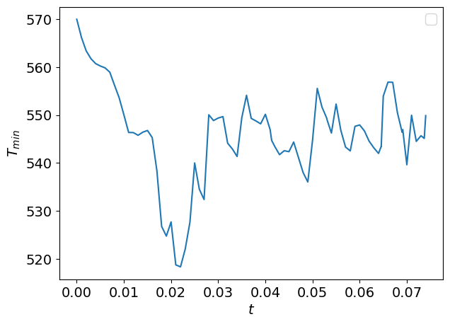
As you can see, the minimal temperature as a function of the time behaves differently before t≈0.03 and after. Indeed, until t≈0.03, the flow is evolving from the initial conditions until the statistically steady state.
For reliable statistics and quantifications of the minimal temperature, we would like to get rid of the warm-up period and find the transient time tt at which the system switches from the warm-up state to the statistically steady state.
Mean and standard deviation of the signal
Before diving into finding the transient time of the signal presented, some mathematical background is needed to explain the methodology.
Let’s imagine a time-dependent signal f(t) where t is the time. This signal is assumed to be extracted from continuous stationary ergordic random processes. We can then define the mean μf and the standard deviation σf of the signal as
where ????[X] is the expected value of X. μf and σf can only be obtained from infinite sample lengths. For a signal of length T=tend−tini where tini and tend are respectively the beginning and end of the signal, μf and σf can be approximated by
For a finite number of samples [f(t0),f(t1),…,f(tn)] with t0<t1<⋯<tn and tn−t0=T, this becomes
If now, we divide the signal f(t) into time-windows of length Tw, the absolute statistical error on the estimate ϕ̂ Tw (=μ̂ Tw or σ̂ Tw) for the time-windows length Tw compared to the estimate ϕ̂ T (respectively μ̂ T or σ̂ T) for the full length of the signal T is given by
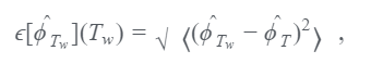
where <> denotes the average over all the time-windows. With this equation, the error as a function of the sample length can be estimated. Note that the accuracy of this error decreases as Tw becomes close to T since fewer windows are available to compute the error. For the case of the bandwidth-limited Gaussian white noise, the error on the estimates μ̂ T and σ̂ T as a function of the sample length Tcan directly be obtained through:
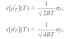
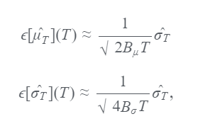
where B is the bandwidth. These approximations are valid for BT≥5. Since σf is not known, this term is replaced by the best standard deviation estimate that is here σ̂ T. Also, to further detect the transient times, the authors of the article decided to use two bandwidth parameters Bμ and Bσ. Thus, the errors in the estimates become:
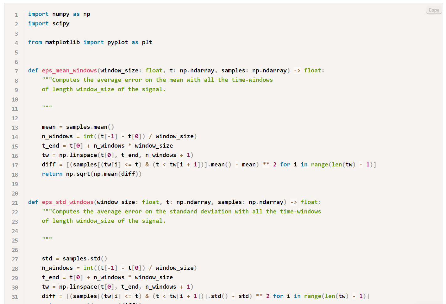
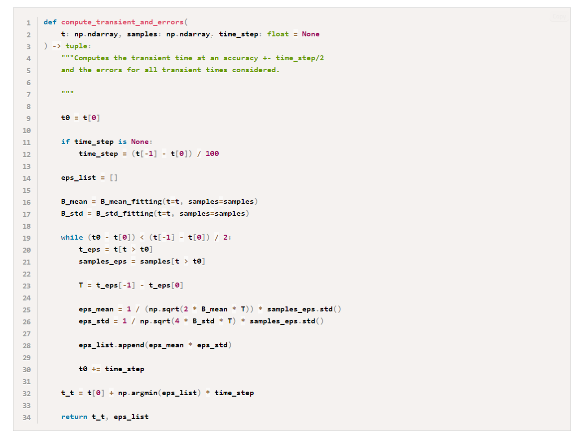
The parameters Bμ and Bσ are obtained as the lowest bandwidth values such as the curves of ϵ[ϕ̂ T](T) intersect the ones of ϵ[ϕ̂ Tw](Tw). Here is the Python program to plot the errors estimated with the windows and with the bandwidth-limited Gaussian white noise:

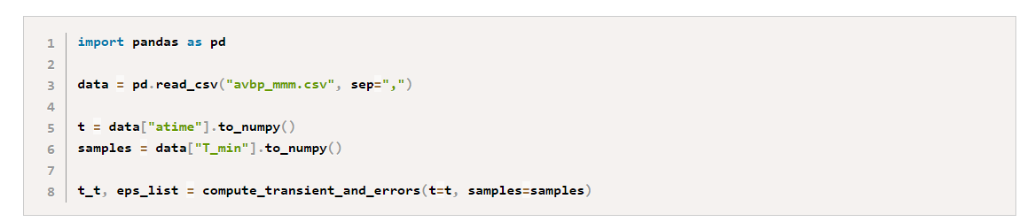
If we go back to the minimal temperature signal presented earlier, by running the following program, we ask this:
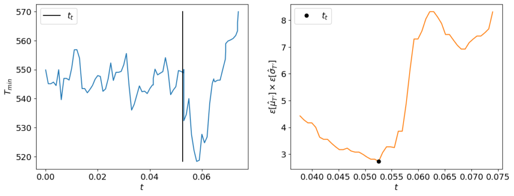
We obtain the following figure:
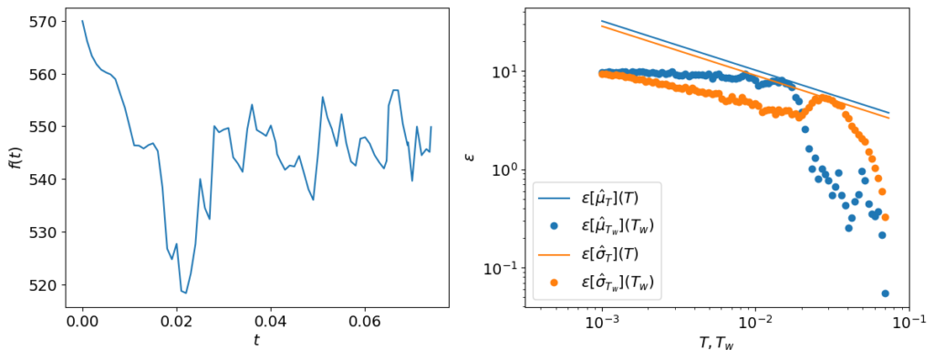
On the left, you can observe the original signal and on the right, the errors of the estimates of the mean and standard deviation with the bandwidth-limited Gaussian white noise formulas and windows estimates. Note that the error predicted with the bandwidth-limited Gaussian white noise is over-estimated compared to the error computed with the time-windows method. Still, since it is often preferable to over-estimate the error than to under-estimate it, this failure will not have a significant impact on the methodology.
Method to detect the transient times
To detect the transient times, the data obtained will successively be shortened starting from a time t≥t0
to obtain a signal of length T′=tn−t. If we call tt the time at which the end of the warm-up period occurs, and Tt=tn−tt
the length of the signal in the statistically steady state, the following hypotheses are considered:
-
for t<tt, the total error ϵ[μ̂ T′]×ϵ[σ̂ T′] (computed with the bandwidth-limited Gaussian noise formulas) is higher than ϵ[μ̂ Tt]×ϵ[σ̂ Tt].. Indeed, the inclusion of the transient period in the computation of the mean and standard deviation is supposed to result in a distortion in at least one of these quantities and increase the errors on these predictions.
-
for t>tt, as we increase t, the total error ϵ[μ̂ T′]×ϵ[σ̂ T′]begins to rise again since the error is inversely proportional to the time period considered.
For these reasons, the transient time is determined by finding T′, such that the total error ϵ[μ̂ T′]×ϵ[σ̂ T′] is minimized. As T′ becomes closer to T,
the statistical estimates become more inaccurate as fewer samples are provided, which results in various local optima in the total error. For this reason, as in the original implementation, we set the limit T′<T/2. The following program will be used to find the transient times and to plot the error as a function of the time t.
Application
Let’s now apply the method to detect the warm-up period on the signal presented!
The output of this program can then be used to build the following plot:
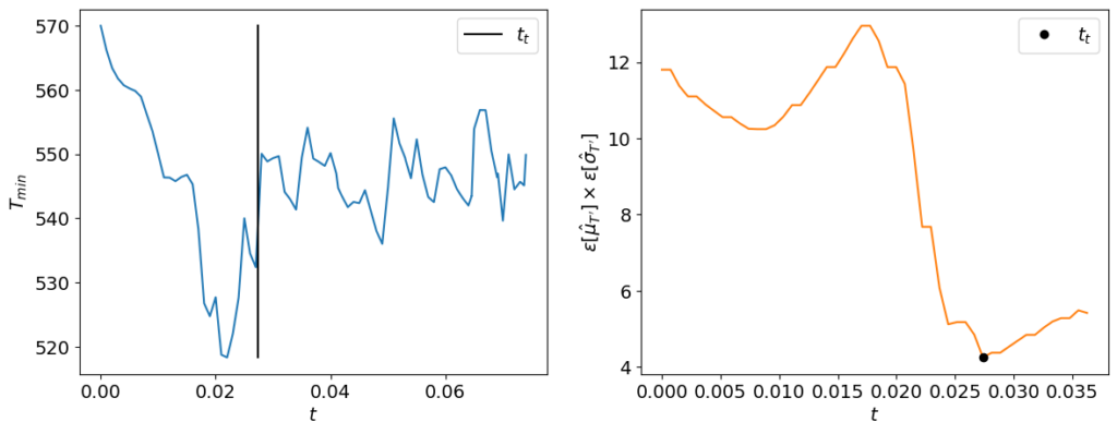
The transient time tt detected with the method is coherent with the visual inspection of the signal (left on the figure). On the right of the figure, you can observe
the total error as a function of the time. The minimum of this curve gives the transient time.
Reverse method
Note that this method can easily be extended to the case where you want to find the end of an initially steady state becoming unsteady (e.g. in an extinction simulation). The method is the same, except that this time we shorten the signal from the ending edge:
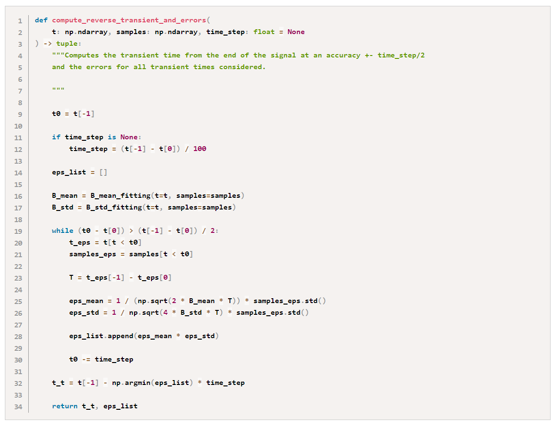
If we flip the original signal and apply this function to the resulting signal, we obtain the following:

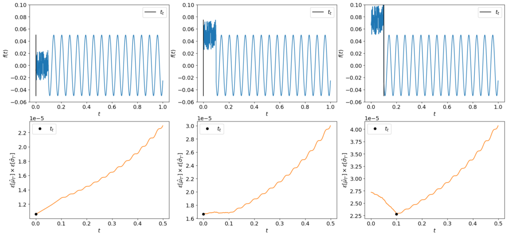
Limitations
We observed however a limitation in this algorithm. Indeed, as said earlier, the warm-up period is supposed to distort the mean or standard deviation compared to the statistically steady state. However, if the signal of the warm-up period remains in the range of amplitudes of the signal of the statistically steady state, the algorithm will not detect the period change. The following examples show this limitation.
Takeaways
In this post, we were interested in detecting the warm-up period in a signal. Despite their limitations previously shown, the Python scripts presented here may help you get rid of this period in a signal and automate your post-treatment for reliable statistics.
The error formulas introduced may also be used to build a workflow that would run until the error of the statistics estimates reaches a certain threshold or that we have an adequate confidence interval of the desired quantity.
Note:
Many thanks to Francesco Salvadore and Antonio Memmolo from CINECA for bringing this article to our attention through their initial FORTRAN implementation conversation. This work is part of the Center of Excellence EXCELLERAT Phase 2, funded by the European Union. This work has received funding from the European High-Performance Computing Joint Undertaking (JU) and Germany, Italy, Slovenia, Spain, Sweden, and France under grant agreement No 101092621.
Authors: Antoine Dauptain, Anthony Larroque, Cerfacs